Plotting with Matplotlib

While UXarray’s plotting API is written around the HoloViz stack of packages, plotting directly with Matplotlib is supported through the conversion to a LineCollection or PolyCollection object. This user guide will cover:

• Converting a Grid to a LineCollection

• Converting a UxDataArray to a PolyCollection

• Using Geographic Projections & Elements

• Handling periodic elements along the antimeridian

import uxarray as ux
import matplotlib.pyplot as plt
import cartopy.crs as ccrs

base_path = "../../test/meshfiles/ugrid/outCSne30/"
grid_path = base_path + "outCSne30.ug"
data_path = base_path + "outCSne30_vortex.nc"

uxds = ux.open_dataset(grid_path, data_path)

Visualize Grid Topology with LineCollection

The Grid.to_linecollection() method can be used to convert a Grid instance into a matplotlib.collections.LineCollection instance. It represents a collection of lines that represent the edges of an unstructured grid.

lc = uxds.uxgrid.to_linecollection()

Once we have converted our Grid to a LineCollection, we can directly use Matplotlib.

# control the width of each edge
lc.set_linewidth(0.5)

# set the color of each edge
lc.set_edgecolor("black")

fig, ax = plt.subplots(1, 1, figsize=(10, 5), constrained_layout=True)

ax.set_xlim((-180, 180))
ax.set_ylim((-90, 90))
ax.add_collection(lc)

plt.title("Line Collection Plot")
plt.show()

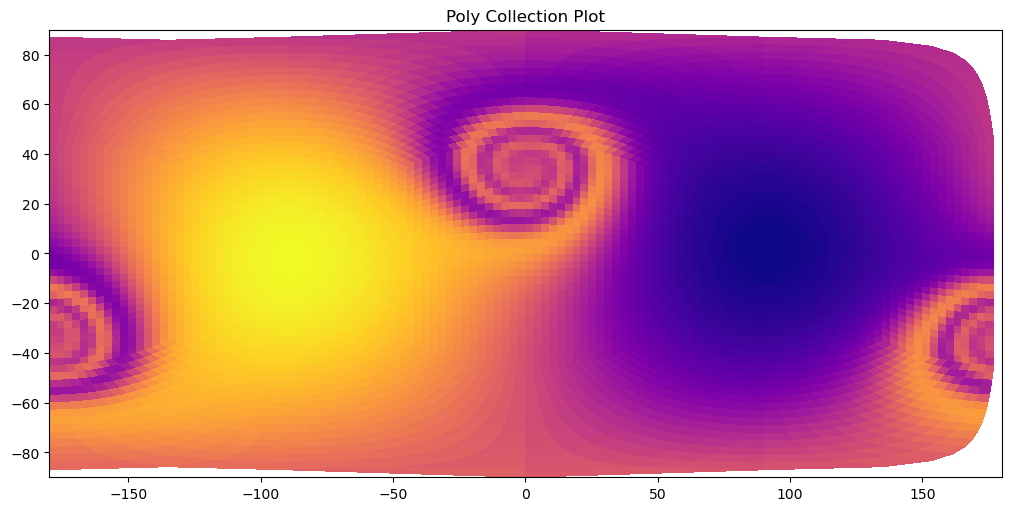
Visualize Data with PolyCollection

The Grid.to_polycollection() method can be used to convert a UxDataArray containing a face-centered data variable into a matplotlib.collections.PolyCollection instance. It represents a collection of polygons that represent the faces of an unstructured grid, shaded using the values of the face-centered data variable.

pc = uxds["psi"].to_polycollection()

Just like with the LineCollection, we can directly use Matplotlib to visualize our PolyCollection

pc.set_antialiased(False)

pc.set_cmap("plasma")

fig, ax = plt.subplots(1, 1, figsize=(10, 5), constrained_layout=True)

ax.set_xlim((-180, 180))
ax.set_ylim((-90, 90))
ax.add_collection(pc)

plt.title("Poly Collection Plot")
plt.show()

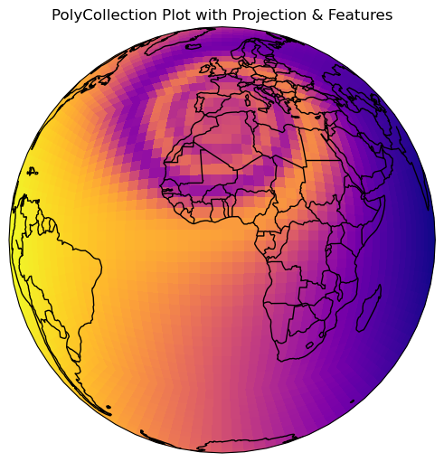
Geographic Projections & Elements

Both the Grid.to_linecollection() and UxDataArray.to_polycollection() methods accept an optional argument projection for setting a Cartopy projection. A full list of Cartopy projections can be found here.

projection = ccrs.Orthographic()

pc = uxds["psi"].to_polycollection(projection=projection, override=True)

import cartopy.feature as cfeature

pc.set_antialiased(False)
pc.set_cmap("plasma")

fig, ax = plt.subplots(
    1,
    1,
    figsize=(10, 5),
    facecolor="w",
    constrained_layout=True,
    subplot_kw=dict(projection=projection),
)

# add geographic features
ax.add_feature(cfeature.COASTLINE)
ax.add_feature(cfeature.BORDERS)

ax.add_collection(pc)
ax.set_global()
plt.title("PolyCollection Plot with Projection & Features")

Text(0.5, 1.0, 'PolyCollection Plot with Projection & Features')

/home/docs/checkouts/readthedocs.org/user_builds/uxarray/conda/v2024.08.0/lib/python3.12/site-packages/cartopy/io/__init__.py:241: DownloadWarning: Downloading: https://naturalearth.s3.amazonaws.com/110m_cultural/ne_110m_admin_0_boundary_lines_land.zip
  warnings.warn(f'Downloading: {url}', DownloadWarning)

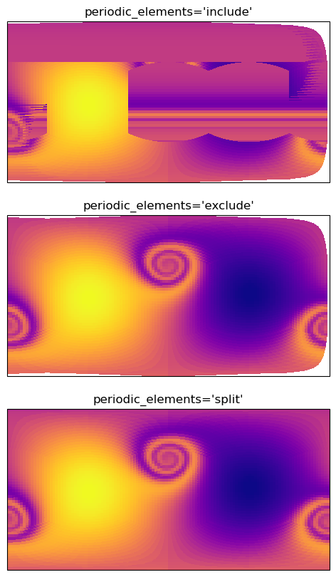
Handling Periodic Elements

Global Data

If your grid contains elements that cross the antimeridian, plotting them without any corrections will lead to artifacts, as can be observed in the first plot below.

UXarray provides two ways of handling these elements:

• Exclusion: Elements will be excluded from the plot, with no other corrections being done, indicated by setting periodic_elements='exclude', this is the default.

• Splitting: Each element is split into two across the antimeridian, indicated by setting periodic_elements='split'

Warning

Setting periodic_elements='split' will lead to roughly a 20 times perfromance hit compared to the other method, so it is suggested to only use this option for small grids.

methods = ["include", "exclude", "split"]
poly_collections = [
    uxds["psi"].to_polycollection(periodic_elements=method) for method in methods
]


fig, axes = plt.subplots(
    nrows=3, figsize=(20, 10), subplot_kw={"projection": ccrs.PlateCarree()}
)

for ax, pc, method in zip(axes, poly_collections, methods):
    pc.set_linewidth(0)
    pc.set_cmap("plasma")
    ax.set_xlim((-180, 180))
    pc.set_antialiased(False)
    ax.set_ylim((-90, 90))
    ax.add_collection(pc)
    ax.set_title(f"periodic_elements='{method}'")

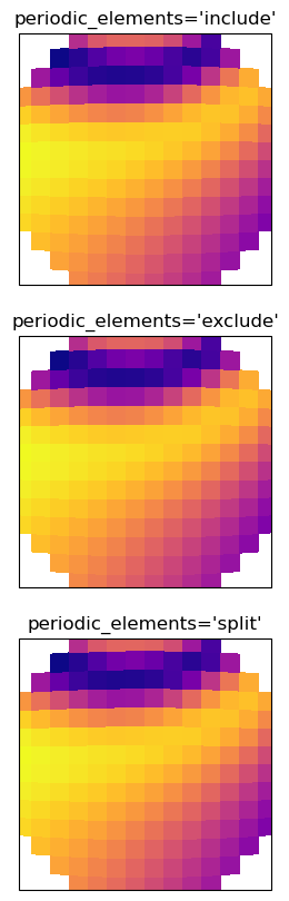
Regional Data

If you grid doesn’t contain any periodic elements, it is always suggested to keep periodic_elements='include' for the best perfromance, as there is no difference in the resulting plots.

methods = ["include", "exclude", "split"]
poly_collections = [
    uxds["psi"]
    .subset.bounding_circle((0, 0), 20)
    .to_polycollection(periodic_elements=method)
    for method in methods
]


fig, axes = plt.subplots(
    nrows=3, figsize=(10, 10), subplot_kw={"projection": ccrs.PlateCarree()}
)

for ax, pc, method in zip(axes, poly_collections, methods):
    pc.set_linewidth(0)
    pc.set_cmap("plasma")
    pc.set_antialiased(False)
    ax.set_xlim((-20, 20))
    ax.set_ylim((-20, 20))
    ax.add_collection(pc)
    ax.set_title(f"periodic_elements='{method}'")