Plotting with Matplotlib and Cartopy#
In addition to supporting the HoloViz ecosystem of plotting packages via the .plot() accessors, UXarray also provides functionality to represent unstructured grids in formats that are accepted by Matplotlib and Cartopy.
This guide covers:
Rasterizing Data onto a Cartopy
GeoAxesVisualizing Data with
PolyCollectionVisualizing Grid Topology
import cartopy.crs as ccrs
import cartopy.feature as cfeature
import matplotlib.pyplot as plt
from cartopy.crs import PlateCarree

import uxarray as ux
uxds = ux.tutorial.open_dataset("mpas-QU-480")
Matplotlib and Cartopy Background#
To support Matplotlib and Cartopy workflows, UXarray has chosen to provide the necessary conversion functions to represent unstructured grids in formats that can be interpreted by these packages. This means that you as the user are responsible for setting up the figure, adding colorbar, and configuring other aspects of the plotting workflow. Because of this, we will not cover these topics in detail, but recommend reviewing the following resources:
Rasterization#
UXarray can rapidly translate face-centered data into a raster image that can be displayed directly on a Cartopy GeoAxes.
UXarray currently supports a nearest-neighbor based rasterization method, which converts each screen-space pixel from the GeoAxes into a geographic coordinate for sampling the underlying unstructured grid. If the pixel lies within a face in the unstructured grid, it is shaded by the corresponding face value.
The result is a 2-D array that works seamlessly with Matplotlib’s imshow, contour, contourf and other visualization functions.
Important
Since the core geometry routines used internally directly sample the underlying unstructured grid using Numba, rasterization is extremely fast, even on high-resolution unstructured grids.
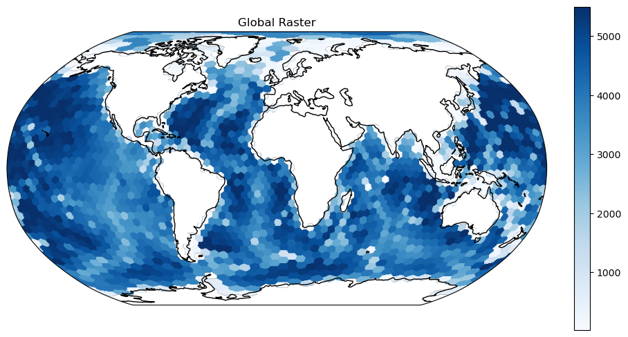
Displaying Rasterized Data with ax.imshow()#
Because rasterization yields a fully georeferenced two-dimensional array, the quickest way to render it is with Matplotlib’s imshow() on a Cartopy GeoAxes. By supplying the raster array along with the appropriate origin and extent parameters, Cartopy automatically handles projection and alignment.
Caution
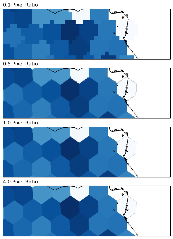
When rasterizing a grid at a global extent, especially for higher-resolution grids, there may not be enough pixels to sample the entire grid thoroughly with the default pixel_ratio of 1.0. You can consider increasing the pixel_ratio if you need more pixels. The impact is demonstrated in an example below.
fig, ax = plt.subplots(
    subplot_kw={"projection": ccrs.Robinson()}, figsize=(9, 6), constrained_layout=True
)

ax.set_global()

raster = uxds["bottomDepth"].to_raster(ax=ax)
img = ax.imshow(
    raster, cmap="Blues", origin="lower", extent=ax.get_xlim() + ax.get_ylim()
)
ax.set_title("Global Raster")
ax.coastlines()

# Adding a colorbar (the examples below will not include one to keep things concise)
cbar = fig.colorbar(img, ax=ax, fraction=0.03)
/home/docs/checkouts/readthedocs.org/user_builds/uxarray/conda/latest/lib/python3.14/site-packages/uxarray/grid/point_in_face.py:168: NumbaPerformanceWarning: np.dot() is faster on contiguous arrays, called on (Array(float64, 1, 'C', False, aligned=True), Array(float64, 1, 'A', False, aligned=True))
  hits = _get_faces_containing_point(
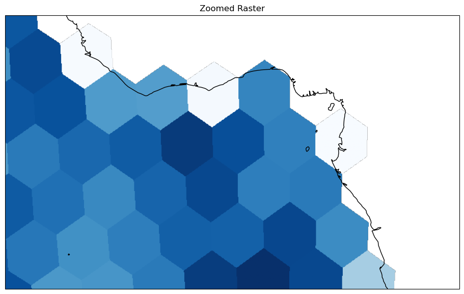
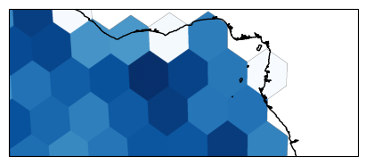
When you only need to visualize a subset of your data, such as a country, basin, or smaller study area, limiting the extent of the Cartopy GeoAxes before rasterization can significantly improve performance. By setting a tighter longitude-latitude window, the pixel-to-face lookups are constrained to that region, reducing the overall number of queries. This targeted sampling speeds up rendering, lowers memory overhead, and produces a cleaner, more focused map of your area of interest.
fig, ax = plt.subplots(
    subplot_kw={"projection": ccrs.Robinson()}, figsize=(9, 6), constrained_layout=True
)

ax.set_extent((-20, 20, -10, 10))


raster = uxds["bottomDepth"].to_raster(ax=ax)
ax.imshow(raster, cmap="Blues", origin="lower", extent=ax.get_xlim() + ax.get_ylim())
ax.set_title("Zoomed Raster")
ax.coastlines()
<cartopy.mpl.feature_artist.FeatureArtist at 0x71ff7d7f9590>
Controlling the resolution#
You can control the resolution of the rasterization by adjusting the pixel_ratio parameter.
A value greater than 1 increases the resolution (sharpens the image), while a value less than 1 will result in a coarser rasterization.
The resolution also depends on what the figure’s DPI setting is prior to calling to_raster().
The pixel_ratio parameter can also be used with the standard HoloViz/Datashader-based plotting
(i.e. the plot() accessor; examples in Plotting).
pixel_ratios = [0.1, 0.5, 1, 4]

fig, axs = plt.subplots(
    len(pixel_ratios),
    1,
    subplot_kw={"projection": ccrs.Robinson()},
    figsize=(6, 8),
    constrained_layout=True,
    sharex=True,
    sharey=True,
)

axs.flat[0].set_extent((-20, 20, -5, 5))

for ax, pixel_ratio in zip(axs.flat, pixel_ratios):
    raster = uxds["bottomDepth"].to_raster(ax=ax, pixel_ratio=pixel_ratio)
    ax.imshow(
        raster, cmap="Blues", origin="lower", extent=ax.get_xlim() + ax.get_ylim()
    )
    ax.set_title(f"{pixel_ratio:.1f} Pixel Ratio", loc="left")
    ax.coastlines()
/home/docs/checkouts/readthedocs.org/user_builds/uxarray/conda/latest/lib/python3.14/site-packages/cartopy/io/__init__.py:242: DownloadWarning: Downloading: https://naturalearth.s3.amazonaws.com/10m_physical/ne_10m_coastline.zip
  warnings.warn(f'Downloading: {url}', DownloadWarning)
Reusing the pixel mapping#
As we see below, this is helpful if you are planning to make multiple plots of the same scene, allowing the raster to be computed much more quickly after the first time.
Use return_pixel_mapping=True to get back the pixel mapping, and then pass it in the next time you call to_raster().
%%time

fig, ax = plt.subplots(
    figsize=(4, 2), subplot_kw={"projection": ccrs.Robinson()}, constrained_layout=True
)

ax.set_extent((-20, 20, -7, 7))

raster, pixel_mapping = uxds["bottomDepth"].to_raster(
    ax=ax, pixel_ratio=5, return_pixel_mapping=True
)
ax.imshow(raster, cmap="Blues", origin="lower", extent=ax.get_xlim() + ax.get_ylim())
ax.coastlines()
CPU times: user 20.2 s, sys: 176 ms, total: 20.4 s
Wall time: 11.5 s
<cartopy.mpl.feature_artist.FeatureArtist at 0x71ff7d162ad0>
pixel_mapping
<xarray.DataArray 'pixel_mapping' (n_pixel: 1193500)> Size: 10MB
array([1385, 1385, 1385, ...,   -1,   -1,   -1], shape=(1193500,))
Dimensions without coordinates: n_pixel
Attributes:
    long_name:    pixel_mapping
    description:  Mapping from raster pixels within a Cartopy GeoAxes to near...
    projection:   +proj=robin +a=6378137.0 +lon_0=0 +no_defs +type=crs
    ax_xlim:      [-1884860.97093615  1884860.97093615]
    ax_ylim:      [-795895.28220694  795895.28220694]
    ax_shape:     [ 770 1550]
pixel_ratio: 5.0%%time
fig, ax = plt.subplots(
figsize=(4, 2), subplot_kw={"projection": ccrs.Robinson()}, constrained_layout=True
)
ax.set_extent((-20, 20, -7, 7))
raster = uxds["bottomDepth"].to_raster(ax=ax, pixel_mapping=pixel_mapping)
ax.imshow(raster, cmap="Blues", origin="lower", extent=ax.get_xlim() + ax.get_ylim())
ax.coastlines()
CPU times: user 285 ms, sys: 11 ms, total: 296 ms
Wall time: 296 ms
<cartopy.mpl.feature_artist.FeatureArtist at 0x71ff85141310>
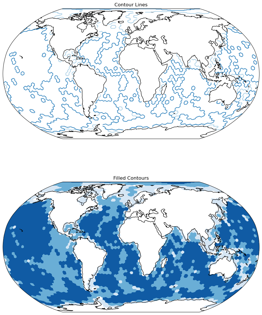
Viewing Contours with ax.contour() and ax.contourf()#
You can use ax.contour() to draw projection-aware isolines and ax.contourf() to shade between levels, specifying either a contour count or explicit thresholds.
Warning
The contours are generated on the raster image, not the unstructured grid geometries, which may create misleading results if not enough pixels were sampled.
levels = [0, 2000, 4000, 6000]
fig, axes = plt.subplots(
    2,
    1,
    subplot_kw={"projection": ccrs.Robinson()},
    constrained_layout=True,
    figsize=(9, 12),
)

ax1, ax2 = axes

ax1.set_global()
ax2.set_global()

ax1.coastlines()
ax2.coastlines()

raster = uxds["bottomDepth"].to_raster(ax=ax1)

# Contour Lines
ax1.contour(
    raster,
    cmap="Blues",
    origin="lower",
    extent=ax1.get_xlim() + ax1.get_ylim(),
    levels=levels,
)
ax1.set_title("Contour Lines")

# Filled Contours
ax2.contourf(
    raster,
    cmap="Blues",
    origin="lower",
    extent=ax2.get_xlim() + ax2.get_ylim(),
    levels=levels,
)
ax2.set_title("Filled Contours")
Text(0.5, 1.0, 'Filled Contours')
Matplotlib Collections#
Instead of directly sampling the unstructured grid, UXarray supports converting the grid into two matplotlib.collections classes: PolyCollection and LineCollection.
Warning
It is recommended to only use these collection-based plotting workflows if your grid is relatively small. For higher-resolution grids, directly rasterizing will almost always produce quicker results.
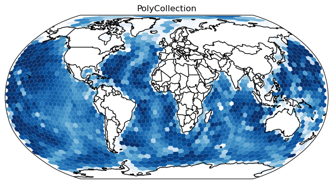
Visualize Data with PolyCollection#
To visualize face-centered data variables, you can convert a UxDataArray into a PolyCollection, which represents each face as a polygon, shaded by its corresponding data value.
projection = ccrs.Robinson()
poly_collection = uxds["bottomDepth"].to_polycollection(projection=projection)
poly_collection.set_cmap("Blues")

fig, ax = plt.subplots(
    1,
    1,
    facecolor="w",
    constrained_layout=True,
    subplot_kw=dict(projection=projection),
)

ax.add_feature(cfeature.COASTLINE)
ax.add_feature(cfeature.BORDERS)

ax.add_collection(poly_collection)
ax.set_global()
plt.title("PolyCollection")
Text(0.5, 1.0, 'PolyCollection')
/home/docs/checkouts/readthedocs.org/user_builds/uxarray/conda/latest/lib/python3.14/site-packages/cartopy/io/__init__.py:242: DownloadWarning: Downloading: https://naturalearth.s3.amazonaws.com/110m_cultural/ne_110m_admin_0_boundary_lines_land.zip
  warnings.warn(f'Downloading: {url}', DownloadWarning)
Important
to_polycollection() defaults to periodic_elements="exclude"; use "split" to preserve antimeridian faces.
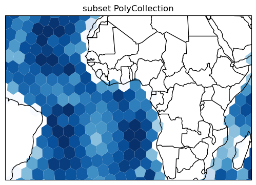
To reduce the number of polygons in the collection, you can subset before converting.
lon_bounds = (-50, 50)
lat_bounds = (-20, 20)
b = 15  # buffer for the selection so we can fill the plot area

poly_collection = (
    uxds["bottomDepth"]
    .subset.bounding_box(
        lon_bounds=(lon_bounds[0] - b, lon_bounds[1] + b),
        lat_bounds=(lat_bounds[0] - b, lat_bounds[1] + b),
    )
    .to_polycollection(projection=projection)
)

poly_collection.set_cmap("Blues")

fig, ax = plt.subplots(
    1,
    1,
    figsize=(7, 3.5),
    facecolor="w",
    constrained_layout=True,
    subplot_kw=dict(projection=projection),
)

ax.set_extent(lon_bounds + lat_bounds)

ax.add_feature(cfeature.COASTLINE)
ax.add_feature(cfeature.BORDERS)

ax.add_collection(poly_collection)
plt.title("subset PolyCollection")
Text(0.5, 1.0, 'subset PolyCollection')
Tip
When working with a fine grid, matplotlib’s anti-alias algorithm can sometimes produce unexpected visualization effects that look like missing patches or a white “hazing” from the fine slivers between the polygons. Try using poly_collection.set_edgecolor('face) and adjusting with poly_collection.set_linewidth() if needed.
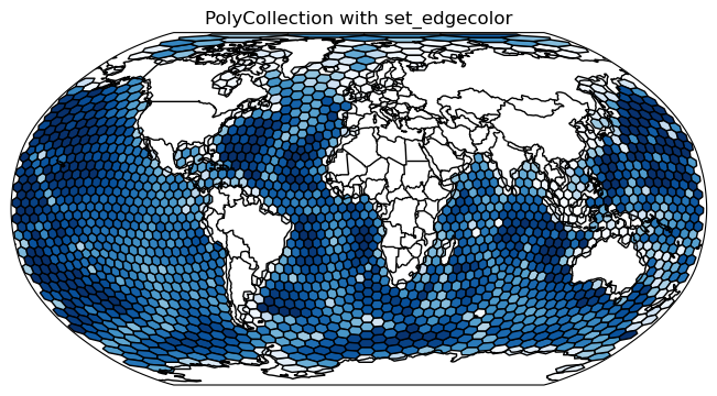
Visualize Grid Topology#
Using PolyCollection#
To visualize the unstructured grid geometry, you can set the edge color on an existing PolyCollection.
projection = ccrs.Robinson()
poly_collection = uxds["bottomDepth"].to_polycollection(projection=projection)

poly_collection.set_cmap("Blues")
poly_collection.set_edgecolor("black")

fig, ax = plt.subplots(
    1,
    1,
    facecolor="w",
    constrained_layout=True,
    subplot_kw=dict(projection=projection),
)

ax.add_feature(cfeature.COASTLINE)
ax.add_feature(cfeature.BORDERS)

ax.add_collection(poly_collection)
ax.set_global()
plt.title("PolyCollection with set_edgecolor")
Text(0.5, 1.0, 'PolyCollection with set_edgecolor')
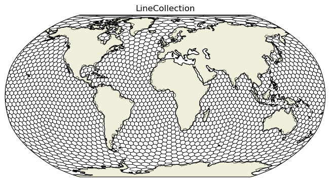
Using LineCollection#
You can also convert a Grid into a LineCollection, which stores the edges of the unstructured grid.
line_collection = uxds.uxgrid.to_linecollection(
    colors="black", linewidths=0.5, periodic_elements="split"
)
fig, ax = plt.subplots(
    1,
    1,
    constrained_layout=True,
    subplot_kw={"projection": ccrs.Robinson()},
)

ax.add_feature(cfeature.LAND)
ax.add_feature(cfeature.COASTLINE)
ax.add_collection(line_collection)
ax.set_global()
ax.set_title("LineCollection")
plt.show()
/home/docs/checkouts/readthedocs.org/user_builds/uxarray/conda/latest/lib/python3.14/site-packages/cartopy/io/__init__.py:242: DownloadWarning: Downloading: https://naturalearth.s3.amazonaws.com/110m_physical/ne_110m_land.zip
  warnings.warn(f'Downloading: {url}', DownloadWarning)