Vector Calculus

Vector Calculus#

Computing and working with vector calculus on unstructured grids is essential for analyzing scalar and vector fields in geoscience. This notebook demonstrates UXarray’s finite-volume implementations and verifies expected identities.

We will showcase:

Gradient of face-centered scalar fields (zonal and meridional components)
Curl of vector fields (including curl of a gradient ≈ 0 and a synthetic vortex)
Divergence of vector fields (including Laplacian as ∇·∇φ, divergence of a vortex ≈ 0, and radial expansion > 0)
Scalar dot gradient (advection term v · ∇q)
Vector calculus identities verification

import holoviews as hv
import numpy as np

import uxarray as ux

hv.extension("bokeh")

ⓘ

1. Gradient (∇φ)#

Background#

The gradient of a scalar field φ gives both the direction of steepest increase and the rate of change in that direction. On unstructured grids, we use the Green–Gauss theorem:

\[ \int_V \nabla\phi \, dV = \oint_{\partial V} \phi \, dS \]

Implementation#

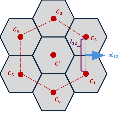
In a finite-volume context, the gradient of a scalar field \(\phi\) is obtained by summing fluxes across each cell face and dividing by the cell’s volume.

Input	Usage	Output
Scalar field \(\phi\)	`φ.gradient()`	Vector field \(\nabla\phi\)

Finite-volume discretization#

\[ \int_V \nabla\phi \, dV = \oint_{\partial V} \phi \, dS \]

Discrete gradient at cell center \(C^*\)#

\[ \nabla\phi(C^*) \;\approx\; \frac{1}{\mathrm{Vol}(C^*)} \sum_{f\in\partial C^*} \left( \frac{\phi(C_i) + \phi(C_j)}{2} \right) \;l_{ij}\;\mathbf{n}_{ij} \]

Plotting Gradients#

To visualize gradients, we represent them as vector fields and overlay them on the original scalar data.

def plot_gradient_vectors(uxda_grad, **kwargs):
    """
    Plots gradient vectors using HoloViews
    """
    uxgrid = uxda_grad.uxgrid
    mag = np.hypot(uxda_grad.zonal_gradient, uxda_grad.meridional_gradient)
    angle = np.arctan2(uxda_grad.meridional_gradient, uxda_grad.zonal_gradient)

    return hv.VectorField(
        (uxgrid.face_lon, uxgrid.face_lat, angle, mag), **kwargs
    ).opts(magnitude="Magnitude")

# Overlay the gradient vector field on top of the original data variable
p1 = (
    uxds["face_lat"].plot(cmap="Oranges", aspect=1) * plot_gradient_vectors(grad_lat)
).opts(title="∇ Cell Latitudes")
p2 = (
    uxds["face_lon"].plot(cmap="Oranges", aspect=1) * plot_gradient_vectors(grad_lon)
).opts(title="∇ Cell Longitudes")
p3 = (
    uxds["gaussian"].plot(cmap="Oranges", aspect=1) * plot_gradient_vectors(grad_gauss)
).opts(title="∇ Gaussian")
p4 = (
    uxds["inverse_gaussian"].plot(cmap="Oranges", aspect=1)
    * plot_gradient_vectors(grad_inv_gauss)
).opts(title="∇ Inverse Gaussian")

# Compose all four plots in a 2 column layout
(p1 + p2 + p3 + p4).cols(2).opts(shared_axes=False)

2. Curl (∇ × F)#

Background#

The curl of a vector field F = (u, v) measures the local rotation or circulation. In 2D, curl produces a scalar field representing the magnitude of rotation:

\[ \text{curl}(\mathbf{F}) = \nabla \times \mathbf{F} = \frac{\partial v}{\partial x} - \frac{\partial u}{\partial y} \]

Positive curl: Counter-clockwise rotation
Negative curl: Clockwise rotation
Zero curl: No local rotation (irrotational flow)

Usage#

Curl can be computed using the UxDataArray.curl() method on vector field components:

Input	Usage	Output
Vector field (u, v)	`u.curl(v)`	Scalar curl field

Constant Fields (Mathematical Validation)#

The curl of a constant vector field should be zero everywhere (within numerical precision).

# Constant vector field: u=1, v=2 (face-centered)
u_constant = uxds["face_lat"] * 0 + 1.0
v_constant = uxds["face_lat"] * 0 + 2.0

# Compute partials via gradient
grad_u = u_constant.gradient()
grad_v = v_constant.gradient()
du_dy = grad_u["meridional_gradient"]
dv_dx = grad_v["zonal_gradient"]
curl_constant = dv_dx - du_dy

finite = np.isfinite(curl_constant.values)
vals = curl_constant.values[finite]
print(
    f"Total faces: {curl_constant.size}, interior: {vals.size}, boundary NaNs: {np.isnan(curl_constant.values).sum()}"
)
if vals.size:
    print(f"Finite curl range: [{vals.min():.2e}, {vals.max():.2e}]")
    print(
        f"Max |curl|: {np.abs(vals).max():.2e}, Mean |curl|: {np.abs(vals).mean():.2e}"
    )

Total faces: 195, interior: 147, boundary NaNs: 48
Finite curl range: [0.00e+00, 0.00e+00]
Max |curl|: 0.00e+00, Mean |curl|: 0.00e+00

Gaussian Fields#

# Use Gaussian fields as vector components
u_gauss = uxds["gaussian"]
v_gauss = uxds["inverse_gaussian"]

# Compute partials via gradient
grad_u = u_gauss.gradient()
grad_v = v_gauss.gradient()
du_dy = grad_u["meridional_gradient"]
dv_dx = grad_v["zonal_gradient"]
curl_gauss = dv_dx - du_dy

finite = np.isfinite(curl_gauss.values)
vals = curl_gauss.values[finite]
print(
    f"Total faces: {curl_gauss.size}, interior: {vals.size}, boundary NaNs: {np.isnan(curl_gauss.values).sum()}"
)
if vals.size:
    print(f"Finite curl range: [{vals.min():.6f}, {vals.max():.6f}]")
    print(f"Mean curl (finite): {vals.mean():.6f}")

Total faces: 195, interior: 147, boundary NaNs: 48
Finite curl range: [-0.000007, 0.000007]
Mean curl (finite): -0.000000

Example 1: Curl of Gradient Field#

In the continuous setting, curl(∇φ) = 0 exactly for any scalar field φ. On an unstructured mesh, however, gradient and curl are independent finite-volume stencils that do not form a discrete de Rham complex, so the identity holds only approximately. The residual is a discretization error — not a bug — and shrinks with grid refinement.

The magnitude of the residual depends on the units. By default gradient()/curl() scale by uxgrid.sphere_radius (Earth ≈ 6.37×10⁶ m), so each derivative picks up a factor of 1/radius. curl(∇φ) applies the gradient stencil twice and therefore carries a factor of 1/radius² (≈ 4×10⁻¹⁴). For the Gaussian field here (φ ~ O(1)) the scaled residual is ~O(10⁻¹³); on the unit sphere (scale_by_radius=False) the same residual is ~O(1–10). Either way it shrinks with refinement.

# Extract gradient components
u_component = grad_gauss.zonal_gradient
v_component = grad_gauss.meridional_gradient

# Compute partial derivatives via gradient()
grad_u = u_component.gradient()
grad_v = v_component.gradient()
du_dy = grad_u["meridional_gradient"]
dv_dx = grad_v["zonal_gradient"]

# Curl = ∂v/∂x - ∂u/∂y
curl_of_gradient = dv_dx - du_dy

print(
    f"Curl of gradient range: [{curl_of_gradient.min().values:.2e}, {curl_of_gradient.max().values:.2e}]"
)
print(f"Mean absolute curl: {abs(curl_of_gradient).mean().values:.2e}")

# Note: values are ~O(1e-13) (per meter^2) with the default radius scaling,
# so we let the color limits autoscale rather than hardcoding them.
curl_plot = curl_of_gradient.plot(cmap="RdBu_r", aspect=1).opts(
    title="Curl of Gradient Field (Should ≈ 0)", colorbar=True
)
curl_plot

Curl of gradient range: [-1.24e-14, 1.15e-14]
Mean absolute curl: 4.79e-15

Example 2: Synthetic Vortex Field#

To better demonstrate curl, let’s create a synthetic rotating vector field (vortex):

# Get face coordinates
face_lon = uxds.uxgrid.face_lon.values
face_lat = uxds.uxgrid.face_lat.values

# Center the coordinates
lon_center = np.mean(face_lon)
lat_center = np.mean(face_lat)

x = face_lon - lon_center
y = face_lat - lat_center

# Create a vortex: u = -y, v = x (pure rotation)
u_vortex_data = -y
v_vortex_data = x

# Create UxDataArrays
u_vortex = ux.UxDataArray(
    u_vortex_data, dims=["n_face"], uxgrid=uxds.uxgrid, name="u_vortex"
)
v_vortex = ux.UxDataArray(
    v_vortex_data, dims=["n_face"], uxgrid=uxds.uxgrid, name="v_vortex"
)

# Compute curl via gradients (default: scaled by sphere_radius -> per meter)
grad_u = u_vortex.gradient()
grad_v = v_vortex.gradient()
du_dy = grad_u["meridional_gradient"]
dv_dx = grad_v["zonal_gradient"]
curl_vortex = dv_dx - du_dy

print(
    f"Vortex curl range: [{curl_vortex.min().values:.2e}, {curl_vortex.max().values:.2e}]"
)
# On the unit sphere this rotation has curl ~2; with the default radius scaling
# the result is that value divided by sphere_radius (positive and roughly uniform).
print(f"Mean vortex curl: {curl_vortex.mean().values:.2e} (positive => rotational)")

Vortex curl range: [1.80e-05, 1.80e-05]
Mean vortex curl: 1.80e-05 (positive => rotational)

# Plot the vortex vector field and its curl
def plot_vector_field(u, v, **kwargs):
    """Plot vector field using HoloViews"""
    uxgrid = u.uxgrid
    mag = np.hypot(u, v)
    angle = np.arctan2(v, u)

    return hv.VectorField(
        (uxgrid.face_lon, uxgrid.face_lat, angle, mag), **kwargs
    ).opts(magnitude="Magnitude")


# Vector field plot
vortex_vectors = plot_vector_field(u_vortex, v_vortex).opts(
    title="Synthetic Vortex Field", aspect=1, arrow_heads=True
)

# Curl magnitude plot
curl_magnitude = curl_vortex.plot(cmap="Reds", aspect=1).opts(
    title="Curl of Vortex Field", colorbar=True
)

(vortex_vectors + curl_magnitude).opts(shared_axes=False)

Example 3: Relative Vorticity from Solid-Body Rotation#

The 2D curl on the sphere is relative vorticity \(\zeta = \partial v/\partial x - \partial u/\partial y\), a quantity meteorologists and oceanographers care about every day. With the default scale_by_radius=True, u.curl(v) returns \(\zeta\) in physical units of \(s^{-1}\).

A clean analytical check is solid-body rotation about the polar axis with angular speed \(\Omega\):

\[ u(\varphi) = \Omega R \cos\varphi, \qquad v = 0 \]

For this flow the relative vorticity on a sphere of radius \(R\) is

\[ \zeta = -\frac{1}{R\cos\varphi}\frac{\partial(u\cos\varphi)}{\partial \varphi} = -2\Omega \sin\varphi. \]

We construct the field on the existing MPAS subset and compare u.curl(v) against this closed form.

OMEGA = 7.292115e-5  # Earth's angular speed (rad/s)
R = uxds.uxgrid.sphere_radius
lat_rad = np.deg2rad(uxds.uxgrid.face_lat.values)

u_sbr_data = OMEGA * R * np.cos(lat_rad)
v_sbr_data = np.zeros_like(u_sbr_data)

u_sbr = ux.UxDataArray(
    u_sbr_data,
    dims=["n_face"],
    uxgrid=uxds.uxgrid,
    name="u_sbr",
    attrs={"units": "m/s"},
)
v_sbr = ux.UxDataArray(
    v_sbr_data,
    dims=["n_face"],
    uxgrid=uxds.uxgrid,
    name="v_sbr",
    attrs={"units": "m/s"},
)

zeta = u_sbr.curl(v_sbr)
zeta_analytic = -2.0 * OMEGA * np.sin(lat_rad)

finite = np.isfinite(zeta.values)
err = np.abs(zeta.values[finite] - zeta_analytic[finite])

print(f"curl units: {zeta.attrs['units']}")
print(f"sphere_radius (m): {R:.3e}")
print(
    f"computed   zeta range: [{zeta.values[finite].min():.3e}, {zeta.values[finite].max():.3e}]  1/s"
)
print(
    f"analytic   zeta range: [{zeta_analytic.min():.3e}, {zeta_analytic.max():.3e}]  1/s"
)
print(f"max |error|: {err.max():.3e}  1/s  (≈ {err.max() / (2 * OMEGA):.1%} of 2Omega)")

curl units: (m/s)/m
sphere_radius (m): 6.371e+06
computed   zeta range: [-4.448e-06, 4.259e-06]  1/s
analytic   zeta range: [-4.844e-06, 5.039e-06]  1/s
max |error|: 8.895e-06  1/s  (≈ 6.1% of 2Omega)

zeta.plot(cmap="RdBu_r", aspect=1).opts(
    title="Relative Vorticity (1/s) — Solid-Body Rotation", colorbar=True
)

3. Divergence (∇ · F)#

Background#

The divergence of a vector field F = (u, v) measures the local expansion or contraction of the field:

\[ \text{div}(\mathbf{F}) = \nabla \cdot \mathbf{F} = \frac{\partial u}{\partial x} + \frac{\partial v}{\partial y} \]

Positive divergence: Expansion (source)
Negative divergence: Contraction (sink)
Zero divergence: Incompressible flow

Usage#

Divergence can be computed using the UxDataArray.divergence() method:

Input	Usage	Output
Vector field (u, v)	`u.divergence(v)`	Scalar divergence field

Constant Fields (Mathematical Validation)#

The divergence of a constant vector field should be zero everywhere (within numerical precision).

# Constant vector field: u=1, v=2 (face-centered)
u_constant = uxds["face_lat"] * 0 + 1.0
v_constant = uxds["face_lat"] * 0 + 2.0

# Compute partials via gradient
grad_u = u_constant.gradient()
grad_v = v_constant.gradient()
du_dx = grad_u["zonal_gradient"]
dv_dy = grad_v["meridional_gradient"]
div_constant = du_dx + dv_dy

finite = np.isfinite(div_constant.values)
vals = div_constant.values[finite]
print(
    f"Total faces: {div_constant.size}, interior: {vals.size}, boundary NaNs: {np.isnan(div_constant.values).sum()}"
)
if vals.size:
    print(f"Finite divergence range: [{vals.min():.2e}, {vals.max():.2e}]")
    print(f"Max |div|: {np.abs(vals).max():.2e}, Mean |div|: {np.abs(vals).mean():.2e}")

Total faces: 195, interior: 147, boundary NaNs: 48
Finite divergence range: [0.00e+00, 0.00e+00]
Max |div|: 0.00e+00, Mean |div|: 0.00e+00

Gaussian Fields#

# Use Gaussian fields as vector components
u_gauss = uxds["gaussian"]
v_gauss = uxds["inverse_gaussian"]

# Compute partials via gradient
grad_u = u_gauss.gradient()
grad_v = v_gauss.gradient()
du_dx = grad_u["zonal_gradient"]
dv_dy = grad_v["meridional_gradient"]
div_gauss = du_dx + dv_dy

finite = np.isfinite(div_gauss.values)
vals = div_gauss.values[finite]
print(
    f"Total faces: {div_gauss.size}, interior: {vals.size}, boundary NaNs: {np.isnan(div_gauss.values).sum()}"
)
if vals.size:
    print(f"Finite divergence range: [{vals.min():.6f}, {vals.max():.6f}]")
    print(f"Mean divergence (finite): {vals.mean():.6f}")

Total faces: 195, interior: 147, boundary NaNs: 48
Finite divergence range: [-0.000007, 0.000007]
Mean divergence (finite): 0.000000

Example 1: Divergence of Gradient Field#

# Compute divergence of the gradient (Laplacian) via partials
# ∇²φ = ∂(∇φ_x)/∂x + ∂(∇φ_y)/∂y
grad_gauss_u = grad_gauss["zonal_gradient"]
grad_gauss_v = grad_gauss["meridional_gradient"]

gxu = grad_gauss_u.gradient()["zonal_gradient"]  # ∂u/∂x
gyv = grad_gauss_v.gradient()["meridional_gradient"]  # ∂v/∂y

div_of_gradient = gxu + gyv

print(
    f"Divergence of gradient range: [{div_of_gradient.min().values:.2e}, {div_of_gradient.max().values:.2e}]"
)
print("This is the Laplacian (∇²) of the original gaussian field")

div_plot = div_of_gradient.plot(cmap="RdBu_r", aspect=1).opts(
    title="Divergence of Gradient (Laplacian)", colorbar=True
)
div_plot

Divergence of gradient range: [-1.49e-10, 2.81e-12]
This is the Laplacian (∇²) of the original gaussian field

Example 2: Divergence of Vortex Field#

Pure rotation should have zero divergence (incompressible):

# Compute divergence of the vortex via gradients: div = ∂u/∂x + ∂v/∂y
grad_u = u_vortex.gradient()
grad_v = v_vortex.gradient()
du_dx = grad_u["zonal_gradient"]
dv_dy = grad_v["meridional_gradient"]
div_vortex = du_dx + dv_dy

print(
    f"Vortex divergence range: [{div_vortex.min().values:.2e}, {div_vortex.max().values:.2e}]"
)
print(f"Mean absolute divergence: {abs(div_vortex).mean().values:.2e}")
print("Pure rotation should have zero divergence")

# Residual is ~O(1e-13) with default radius scaling; let color limits autoscale.
div_vortex_plot = div_vortex.plot(cmap="RdBu_r", aspect=1).opts(
    title="Divergence of Vortex (Should ≈ 0)", colorbar=True
)
div_vortex_plot

Vortex divergence range: [-2.83e-10, 2.52e-10]
Mean absolute divergence: 9.02e-11
Pure rotation should have zero divergence

Example 3: Radial Expansion Field#

Let’s create a field that expands radially outward to demonstrate positive divergence:

# Create radial expansion field: u = x, v = y
u_radial_data = x
v_radial_data = y

u_radial = ux.UxDataArray(
    u_radial_data, dims=["n_face"], uxgrid=uxds.uxgrid, name="u_radial"
)
v_radial = ux.UxDataArray(
    v_radial_data, dims=["n_face"], uxgrid=uxds.uxgrid, name="v_radial"
)

# Compute curl and divergence via gradients (default: scaled by sphere_radius)
grad_u = u_radial.gradient()
grad_v = v_radial.gradient()
du_dy = grad_u["meridional_gradient"]
dv_dx = grad_v["zonal_gradient"]
du_dx = grad_u["zonal_gradient"]
dv_dy = grad_v["meridional_gradient"]

curl_radial = dv_dx - du_dy
div_radial = du_dx + dv_dy

print(
    f"Radial field curl range: [{curl_radial.min().values:.2e}, {curl_radial.max().values:.2e}]"
)
print(
    f"Radial field divergence range: [{div_radial.min().values:.2e}, {div_radial.max().values:.2e}]"
)
# On the unit sphere this expansion has curl ~0 and divergence ~2; with the
# default radius scaling both are divided by sphere_radius.
print(
    "Expected (unit sphere): curl ≈ 0, divergence ≈ 2; scaled values are /radius smaller"
)

Radial field curl range: [-2.52e-10, 2.83e-10]
Radial field divergence range: [1.80e-05, 1.80e-05]
Expected (unit sphere): curl ≈ 0, divergence ≈ 2; scaled values are /radius smaller

# Plot radial expansion field and its divergence
radial_vectors = plot_vector_field(u_radial, v_radial).opts(
    title="Radial Expansion Field", aspect=1, arrow_heads=True
)

radial_div = div_radial.plot(cmap="Reds", aspect=1).opts(
    title="Divergence of Radial Field", colorbar=True
)

(radial_vectors + radial_div).opts(shared_axes=False)

5. Vector Calculus Identities#

Let’s verify some fundamental vector calculus identities using our computed fields:

Identity 1: Curl of Gradient (Discretization Residual)#

In the continuous setting: ∇ × (∇φ) = 0. UXarray’s finite-volume operators are not mimetic, so this holds only approximately. The residual below is discretization error, not a numerical bug. With the default radius scaling it is ~O(10⁻¹³) for this φ ~ O(1) field (the curl stencil applies a 1/radius² factor); on the unit sphere it is ~O(1–10). It shrinks with grid refinement.

# We already computed this above
max_curl_grad = np.abs(curl_of_gradient).max().values
print(f"Maximum |curl(∇φ)|: {max_curl_grad:.2e}")
print(
    "Note: non-zero residual is expected discretization error from independent "
    "finite-volume gradient and curl stencils (not a bug). Shrinks with grid refinement."
)

Maximum |curl(∇φ)|: 1.24e-14
Note: non-zero residual is expected discretization error from independent finite-volume gradient and curl stencils (not a bug). Shrinks with grid refinement.

Identity 2: Divergence of Curl is Zero#

For any vector field F: ∇ · (∇ × F) = 0

Note: This identity applies to 3D vector fields. In 2D, curl produces a scalar, so we can’t directly compute its divergence.

Identity 3: Properties of Special Fields#

# Summary of field properties
print("Field Properties Summary:")
print("=" * 50)
print("Gradient field:")
print(f"  - Curl: {np.abs(curl_of_gradient).max().values:.2e} (≈ 0, conservative)")
print(
    f"  - Divergence: {div_of_gradient.min().values:.2e} to {div_of_gradient.max().values:.2e} (Laplacian)"
)
print()
print("Vortex field (pure rotation):")
print(f"  - Curl: {curl_vortex.mean().values:.2e} (> 0, rotational)")
print(f"  - Divergence: {np.abs(div_vortex).max().values:.2e} (≈ 0, incompressible)")
print()
print("Radial field (pure expansion):")
print(f"  - Curl: {np.abs(curl_radial).max().values:.2e} (≈ 0, irrotational)")
print(f"  - Divergence: {div_radial.mean().values:.2e} (> 0, expanding)")

Field Properties Summary:
==================================================
Gradient field:
  - Curl: 1.24e-14 (≈ 0, conservative)
  - Divergence: -1.49e-10 to 2.81e-12 (Laplacian)

Vortex field (pure rotation):
  - Curl: 1.80e-05 (> 0, rotational)
  - Divergence: 2.83e-10 (≈ 0, incompressible)

Radial field (pure expansion):
  - Curl: 2.83e-10 (≈ 0, irrotational)
  - Divergence: 1.80e-05 (> 0, expanding)

Vector Calculus

Contents

Vector Calculus#

Data#

1. Gradient (∇φ)#

Background#

Implementation#

Finite-volume discretization#

Discrete gradient at cell center \(C^*\)#

Usage#

Plotting Gradients#

2. Curl (∇ × F)#

Background#

Usage#

Constant Fields (Mathematical Validation)#

Gaussian Fields#

Example 1: Curl of Gradient Field#

Example 2: Synthetic Vortex Field#

Example 3: Relative Vorticity from Solid-Body Rotation#

3. Divergence (∇ · F)#

Background#

Usage#

Constant Fields (Mathematical Validation)#

Gaussian Fields#

Example 1: Divergence of Gradient Field#

Example 2: Divergence of Vortex Field#

Example 3: Radial Expansion Field#

4. Scalar Dot Gradient (v · ∇q)#

Background#

Usage#

5. Vector Calculus Identities#

Identity 1: Curl of Gradient (Discretization Residual)#

Identity 2: Divergence of Curl is Zero#

Identity 3: Properties of Special Fields#